Mass spectrometry fundamentals
How Mass Spectrometry Sensitivity Improved: From Femtomoles to Single Cells
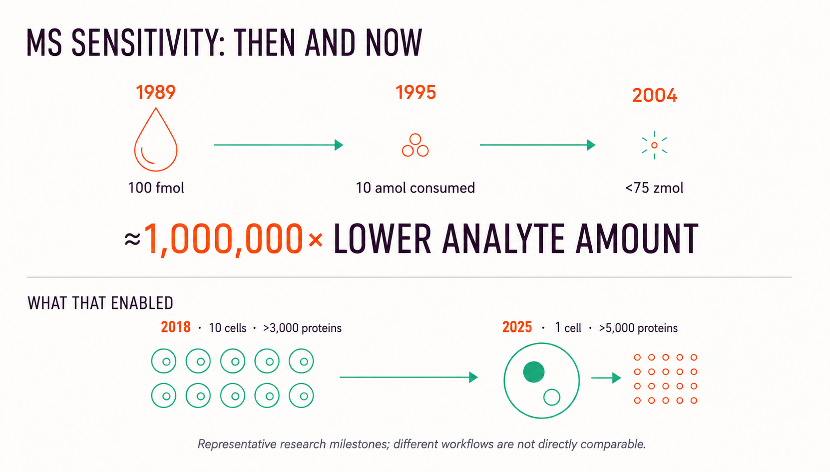
In 1989, electrospray protein analysis typically required roughly 100 femtomoles to 10 picomoles. Fifteen years later, optimized nanoLC–nanoESI–FTICR experiments demonstrated protein identification below 75 zeptomoles. Today, complete workflows can identify more than 5,000 proteins from one mammalian cell. The remarkable part is that no single component produced this progress.
≈106×
The minimum analyte amount in selected biomolecular research demonstrations fell by about six orders of magnitude between the 1989 femtomole milestone and the 2004 sub-75-zeptomole milestone. This is a useful illustration—not a universal specification. Different analytes, instruments, scan modes and definitions of detection were used.


For scale, some optimized targeted LC–MS methods operate in the low-parts-per-trillion range. Twenty ppt by volume is roughly equivalent to distributing one ordinary 50 µL drop throughout an Olympic-size swimming pool. Whether an analyte can actually be detected at that level depends on its ionization efficiency, extraction recovery, matrix suppression, chromatographic peak shape and the measurement mode.
First: “sensitivity” is not one number
A mass spectrometer does not detect concentration directly. It detects ions. Between an analyte molecule in the vial and a recorded peak, the method must retain the molecule during preparation, deliver it chromatographically, ionize it, transmit the ion through the atmospheric-pressure interface, select or accumulate it, measure it and distinguish it from noise.
Consequently, at least five different quantities are often called sensitivity:
- Response or slope: signal change per unit concentration or amount.
- Instrument detection limit (IDL): a test under tightly defined conditions, often using a clean standard.
- Method LOD or LLOQ: the lowest defensible detection or quantification level after extraction and in the real matrix.
- Amount loaded versus amount consumed: especially important for direct infusion and low-flow sources.
- Biological depth: peptides, proteins or metabolites identified from a limited sample such as one cell.
The sensitivity timeline
1978–1988: sensitivity through selectivity
The first working triple-quadrupole instruments established a principle that still dominates quantitative LC–MS/MS: sensitivity can improve by rejecting everything except a chosen precursor-to-product transition. Yost and Enke’s 1978 tandem-quadrupole report and their detailed 1979 treatment laid the foundation for selected-reaction monitoring (SRM). The detector did not suddenly receive every ion; rather, chemical background was removed before the final measurement. In complex samples, that can matter as much as raw ion current.
1989: electrospray opens proteins to routine MS
Electrospray ionization (ESI) changed the analyte universe. Fenn and colleagues showed that large biomolecules could be transferred from solution as multiply charged gas-phase ions. In the same year, Smith and co-workers reported protein analysis on a quadrupole instrument and described sample requirements of 100 fmol to 10 pmol. That range is the first quantitative anchor in Figure 1—not because it defines every 1989 instrument, but because it documents what an influential early ESI workflow could achieve.
1995–1999: nanoelectrospray and better ion transmission
In 1995, Valaskovic and co-workers coupled etched microcapillary emitters to FTMS. Full spectra were obtained from 216 amol loaded, with approximately 10 amol consumed and a reported signal-to-noise ratio of 60:1. A year later, Wilm and Mann formalized nanoelectrospray using 1–2 µm tips and approximately 20 nL/min flow. Smaller droplets improved ionization and desolvation while consuming far less sample.
The atmospheric-pressure interface remained a major loss point. The electrodynamic ion funnel addressed it by focusing collisionally damped ions with RF and DC fields. In a 1998 evaluation, Shaffer and colleagues reported well over one order of magnitude more protein signal than a conventional capillary–skimmer interface under similar conditions. This is the kind of gain that later became embedded inside commercial platforms and disappeared from view as a standalone feature.
2004: the zeptomole demonstration
Shen and colleagues combined micro-SPE, a 15 µm internal-diameter nanoLC column operated near 20 nL/min, nanospray and an 11.4-T FTICR instrument. The integrated platform enabled protein identifications from 0.5 pg of whole-proteome extract and demonstrated identification of individual proteins below 75 zeptomoles.
Using the low end of the 1989 range, 100 fmol divided by 75 zmol is approximately 1.33 million. That is the origin of the “≈1,000,000× lower amount” statement in Figure 1. It should not be read as “a 2004 mass spectrometer was exactly one million times more sensitive than a 1989 mass spectrometer.” The separation, flow rate, ion source, transmission, analyzer and data strategy all changed together.
2005–2015: high resolution without giving up LC timescales
The commercial hybrid linear ion trap–Orbitrap demonstrated that high resolving power and accurate mass could operate on chromatographic timescales. The 2006 evaluation reported nominal resolving power of 60,000 at one spectrum per second, sub-2-ppm accuracy with internal calibration and automatic gain control. High resolution does not automatically create more ions, but it separates analyte signal from isobaric background. Parallel ion accumulation, faster scanning and improved duty cycles later made a larger fraction of a narrow LC peak analytically useful.
2018–today: the workflow becomes the instrument
At trace levels, surfaces can remove more analyte than the mass spectrometer fails to detect. The 2018 nanoPOTS platform reduced preparation volumes below 200 nL to minimize adsorption losses. Coupled to ultrasensitive LC–MS, it identified roughly 1,500–3,000 proteins from about 10–140 cells; with match-between-runs, more than 3,000 proteins were reported from as few as 10 cells.
Single-cell proteomics then combined low-loss handling, multiplexing, narrow-window or data-independent acquisition and faster analyzers. SCoPE-MS and SCoPE2 moved single-cell protein quantification beyond 1,000 proteins per cell. In 2025, the Chip-Tip workflow reported a median of 5,204 proteins from individual HeLa cells and more than 6,000 in one preparation; the method combined nanoliter sample processing, low-flow LC, narrow-window DIA and an Orbitrap Astral instrument. At higher-throughput settings, more than 4,500 proteins per cell were still identified at 80 or 120 samples per day.
| Milestone | Reported result | Main sensitivity lever | What it does not prove |
|---|---|---|---|
| Early ESI protein MS, 1989 | 100 fmol–10 pmol | Soft ionization of multiply charged proteins | A universal 1989 LOD |
| Micro-ESI FTMS, 1995 | ~10 amol consumed | Very low consumption plus high-resolution detection | Routine matrix LLOQ |
| Nanoscale proteomics, 2004 | <75 zmol for an individual protein | Integrated micro-SPE–nanoLC–nanoESI–FTICR workflow | Equal response for every protein |
| nanoPOTS, 2018 | >3,000 proteins from ~10 cells with MBR | Low-loss nanodroplet processing | 3,000 direct MS/MS identifications in every cell |
| Chip-Tip, 2025 | >5,000 proteins in individual HeLa cells | Nearly lossless preparation, low-flow LC, nDIA and fast HRMS | A standalone analyzer detection limit |
Eight engineering changes behind the gain
- Better ionization. ESI and MALDI made intact, nonvolatile biomolecules accessible. NanoESI improved the ratio of ions produced to sample consumed.
- Lower flow and smaller peaks. NanoLC concentrates the same amount into a smaller elution volume and delivers it at a flow regime favorable to electrospray.
- Higher ion transmission. Heated capillaries, ion funnels, RF guides and optimized vacuum interfaces capture more of the spray plume.
- More selective measurement. SRM/MRM, PRM and narrow isolation windows suppress chemical background.
- Faster, more efficient acquisition. Parallel accumulation, shorter transients where appropriate, improved collision cells and faster electronics sample more of each LC peak.
- High resolving power and mass accuracy. Separating an analyte from nearby background improves usable signal-to-noise even without increasing ion production.
- Lower-loss sample preparation. Nanoliter reactors, low-bind surfaces and fewer transfers preserve scarce molecules before they reach the source.
- Better algorithms. DIA extraction, library-free searching and stronger false-discovery control recover confident information from weak but structured signals. Software cannot create missing ions, but it can waste fewer of the ions that were measured.
How to compare the sensitivity of two MS systems
A fair comparison keeps the whole experiment constant. If a vendor application uses a different column, gradient, injection volume, source flow, transition, resolution or peak-integration rule, the result is a workflow comparison—not an analyzer comparison.
- Same analyte, matrix, calibration model and sample-preparation recovery
- Same amount on-column—not merely the same vial concentration
- Same LC peak width, flow rate and injection volume
- Same polarity, adduct, source conditions and acquisition mode
- Same resolving power, scan speed or dwell-time constraint
- Same LOD/LLOQ rule, replicate count and acceptance criteria
- Carryover, blank response and precision included
- Performance checked over a real sequence, not one fresh-source injection
For quantitative bioanalysis, a modern triple quadrupole may outperform an HRMS platform for a predetermined transition because two stages of filtering efficiently reject background. For discovery proteomics or non-target screening, high resolution and acquisition speed may produce more useful sensitivity because the goal is to distinguish thousands of precursors. “Most sensitive” only has meaning after the analytical task is specified.
What limits sensitivity now?
The modern bottleneck is increasingly the probability that a molecule survives the entire workflow. Trace analytes may adsorb to plastic or glass, fail to elute, be ion-suppressed, miss the inlet, be discarded by quadrupole isolation, arrive outside the selected duty cycle or remain indistinguishable from background. Each step can be efficient while the product of all efficiencies remains small.
There is also a speed–sensitivity trade-off. More accumulation time can collect more ions, but reduces the number of measurements across a chromatographic peak. Narrow DIA windows lower interference, but increase the number of windows that must be scanned. Higher resolving power may improve selectivity, but longer transients can reduce throughput. The optimum is rarely the maximum setting.
The next large gains will therefore come from integration: more efficient atmospheric-pressure sampling, lower-flow robust chromatography, genuinely low-loss automation, smarter real-time acquisition and statistical methods designed for sparse ion counts. The lesson of the past 35 years is clear: sensitivity advances fastest when the entire path from sample to decision is redesigned.
Bottom line
Selected literature milestones show a shift from roughly 100-fmol protein requirements in early ESI work to sub-75-zmol demonstrations in optimized nanoscale workflows—a reduction of about six orders of magnitude. Modern single-cell proteomics shows what those accumulated gains enable: thousands of proteins measured from one cell.
But the improvement belongs to the workflow, not to a single analyzer. Ionization, chromatography, transmission, acquisition, surfaces and software all contributed. When evaluating a new MS system, ask not only “What is the detection limit?” but “Under which matrix, workflow, duty cycle and acceptance criteria?” That question turns a spectacular sensitivity claim into useful analytical evidence.
References
- Yost, R. A.; Enke, C. G. Selected ion fragmentation with a tandem quadrupole mass spectrometer. J. Am. Chem. Soc. 1978, 100, 2274–2275. DOI: 10.1021/ja00475a072.
- Fenn, J. B. et al. Electrospray ionization for mass spectrometry of large biomolecules. Science 1989, 246, 64–71. DOI: 10.1126/science.2675315.
- Smith, R. D. et al. Peptide and protein analysis by electrospray ionization-mass spectrometry and capillary electrophoresis-mass spectrometry. Anal. Biochem. 1989, 179, 404–412. DOI: 10.1016/0003-2697(89)90153-X.
- Valaskovic, G. A.; Kelleher, N. L.; Little, D. P.; Aaserud, D. J.; McLafferty, F. W. Attomole-sensitivity electrospray source for large-molecule mass spectrometry. Anal. Chem. 1995, 67, 3802–3805. DOI: 10.1021/ac00116a030.
- Wilm, M.; Mann, M. Analytical properties of the nanoelectrospray ion source. Anal. Chem. 1996, 68, 1–8. DOI: 10.1021/ac9509519.
- Shaffer, S. A. et al. An ion funnel interface for improved ion focusing and sensitivity using electrospray ionization mass spectrometry. Anal. Chem. 1998, 70, 4111–4119. DOI: 10.1021/ac9802170.
- Shen, Y. et al. Ultrasensitive proteomics using high-efficiency online micro-SPE–nanoLC–nanoESI MS and MS/MS. Anal. Chem. 2004, 76, 144–154. DOI: 10.1021/ac030096q.
- Makarov, A. et al. Performance evaluation of a hybrid linear ion trap/Orbitrap mass spectrometer. Anal. Chem. 2006, 78, 2113–2120. DOI: 10.1021/ac0518811.
- Budnik, B. et al. SCoPE-MS: mass spectrometry of single mammalian cells quantifies proteome heterogeneity during cell differentiation. Genome Biol. 2018, 19, 161. DOI: 10.1186/s13059-018-1547-5.
- Zhu, Y. et al. Nanodroplet processing platform for deep and quantitative proteome profiling of 10–100 mammalian cells. Nat. Commun. 2018, 9, 882. DOI: 10.1038/s41467-018-03367-w.
- Specht, H. et al. Single-cell proteomic and transcriptomic analysis of macrophage heterogeneity using SCoPE2. Genome Biol. 2021, 22, 50. DOI: 10.1186/s13059-021-02267-5.
- Li, C. et al. Towards higher sensitivity of mass spectrometry: a perspective from the mass analyzers. Front. Chem. 2021, 9, 813359. DOI: 10.3389/fchem.2021.813359.
- Ye, Z. et al. Enhanced sensitivity and scalability with a Chip-Tip workflow enables deep single-cell proteomics. Nat. Methods 2025, 22, 499–509. DOI: 10.1038/s41592-024-02558-2.
Editorial note: Figure 1 is an original LC–MS Guide illustration. Numerical values were redrawn from the cited publications; no publisher or manufacturer figure was reproduced.
Leave a Reply